Data Transformation

Introduction

It’s very rare that data arrive in exactly the right form you need. Often, you’ll need to create some new variables or summaries, or maybe you just want to rename the variables or reorder the observations to make the data a little easier to work with.

You’ll learn how to do all that (and more!) in this chapter, which will introduce you to data transformation using the polars package and a new dataset on flights that departed New York City in 2013.

The goal of this chapter is to give you an overview of all the key tools for transforming a data frame, a special kind of object that holds tabular data.

We’ll come back these functions in more detail in later chapters, as we start to dig into specific types of data (e.g. numbers, strings, dates).

Prerequisites

In this chapter we’ll focus on the polars package, one of the most widely used tools for data science. You’ll need to ensure you have polars installed. To do this, you can run

import polars as pl

If this command fails, you don’t have polars installed. Open up the terminal in Visual Studio Code (Terminal -> New Terminal), cd to the folder you are working in, and type in uv add polars.

Furthermore, if you wish to check which version of polars you’re using, it’s

pl.__version__

'1.19.0'

You’ll also need the data. Most of the time, data will need to be loaded from a file or the internet. These data are no different, but one of the amazing things about polars is how many different types of data it can load, including from files on the internet.

The data is around 50MB in size so you will need a good internet connection or a little patience for it to download.

Let’s download the data:

import io

import requests

url = "https://raw.githubusercontent.com/byuidatascience/data4python4ds/master/data-raw/flights/flights.csv"
resp = requests.get(url, timeout=60)
resp.raise_for_status()

flights = pl.read_csv(
    io.BytesIO(resp.content),
    null_values=["NA"],
    truncate_ragged_lines=True,
    ignore_errors=True,
)

If the above code worked, then you’ve downloaded the data in CSV format and put it in a data frame. Let’s look at the first few rows using the .head() function that works on all polars data frames.

flights.head()

shape: (5, 19)

year	month	day	dep_time	sched_dep_time	dep_delay	arr_time	sched_arr_time	arr_delay	carrier	flight	tailnum	origin	dest	air_time	distance	hour	minute	time_hour
i64	i64	i64	i64	i64	i64	i64	i64	i64	str	i64	str	str	str	i64	i64	i64	i64	str
2013	1	1	517	515	2	830	819	11	"UA"	1545	"N14228"	"EWR"	"IAH"	227	1400	5	15	"2013-01-01T10:00:00Z"
2013	1	1	533	529	4	850	830	20	"UA"	1714	"N24211"	"LGA"	"IAH"	227	1416	5	29	"2013-01-01T10:00:00Z"
2013	1	1	542	540	2	923	850	33	"AA"	1141	"N619AA"	"JFK"	"MIA"	160	1089	5	40	"2013-01-01T10:00:00Z"
2013	1	1	544	545	-1	1004	1022	-18	"B6"	725	"N804JB"	"JFK"	"BQN"	183	1576	5	45	"2013-01-01T10:00:00Z"
2013	1	1	554	600	-6	812	837	-25	"DL"	461	"N668DN"	"LGA"	"ATL"	116	762	6	0	"2013-01-01T11:00:00Z"

To get more general information on the columns, the data types (dtypes) of the columns, and the size of the dataset, use .glimpse().

flights.glimpse(max_items_per_column=5)

Rows: 336776
Columns: 19
$ year           <i64> 2013, 2013, 2013, 2013, 2013
$ month          <i64> 1, 1, 1, 1, 1
$ day            <i64> 1, 1, 1, 1, 1
$ dep_time       <i64> 517, 533, 542, 544, 554
$ sched_dep_time <i64> 515, 529, 540, 545, 600
$ dep_delay      <i64> 2, 4, 2, -1, -6
$ arr_time       <i64> 830, 850, 923, 1004, 812
$ sched_arr_time <i64> 819, 830, 850, 1022, 837
$ arr_delay      <i64> 11, 20, 33, -18, -25
$ carrier        <str> 'UA', 'UA', 'AA', 'B6', 'DL'
$ flight         <i64> 1545, 1714, 1141, 725, 461
$ tailnum        <str> 'N14228', 'N24211', 'N619AA', 'N804JB', 'N668DN'
$ origin         <str> 'EWR', 'LGA', 'JFK', 'JFK', 'LGA'
$ dest           <str> 'IAH', 'IAH', 'MIA', 'BQN', 'ATL'
$ air_time       <i64> 227, 227, 160, 183, 116
$ distance       <i64> 1400, 1416, 1089, 1576, 762
$ hour           <i64> 5, 5, 5, 5, 6
$ minute         <i64> 15, 29, 40, 45, 0
$ time_hour      <str> '2013-01-01T10:00:00Z', '2013-01-01T10:00:00Z', '2013-01-01T10:00:00Z', '2013-01-01T10:00:00Z', '2013-01-01T11:00:00Z'

You might have noticed the short abbreviations that appear in the dtype column. These tell you the type of the values in their respective columns: i64 is short for integer (eg whole numbers) and f64 is short for double-precision floating point number (these are real numbers). polars has an object data type which allows storing arbitrary Python objects, but this makes you lose performance benefits, as polars is strictly typed. Although not found here, other data types include str for text and datetime for combinations of a date and time.

The table below gives some of the most common data types you are likely to encounter.

Name of data type	Type of data
Float64	real numbers
Categorical	categories
Datetime	date and time
Date	date
Int64	integers
Boolean	True or False
String	text

The different column data types are important because the operations you can perform on a column depend so much on its “type”; for example, you can remove all punctuation from strings while you can multiply ints and floats.

We would like to work with the "time_hour" variable in the form of a datetime; fortunately, polars makes it easy to perform that conversion on that specific column

flights.get_column("time_hour")

shape: (336_776,)

time_hour
str
"2013-01-01T10:00:00Z"
"2013-01-01T10:00:00Z"
"2013-01-01T10:00:00Z"
"2013-01-01T10:00:00Z"
"2013-01-01T11:00:00Z"
…
"2013-09-30T18:00:00Z"
"2013-10-01T02:00:00Z"
"2013-09-30T16:00:00Z"
"2013-09-30T15:00:00Z"
"2013-09-30T12:00:00Z"

flights.with_columns(pl.col("time_hour").str.to_datetime(time_zone="UTC"))

shape: (336_776, 19)

year	month	day	dep_time	sched_dep_time	dep_delay	arr_time	sched_arr_time	arr_delay	carrier	flight	tailnum	origin	dest	air_time	distance	hour	minute	time_hour
i64	i64	i64	i64	i64	i64	i64	i64	i64	str	i64	str	str	str	i64	i64	i64	i64	datetime[μs, UTC]
2013	1	1	517	515	2	830	819	11	"UA"	1545	"N14228"	"EWR"	"IAH"	227	1400	5	15	2013-01-01 10:00:00 UTC
2013	1	1	533	529	4	850	830	20	"UA"	1714	"N24211"	"LGA"	"IAH"	227	1416	5	29	2013-01-01 10:00:00 UTC
2013	1	1	542	540	2	923	850	33	"AA"	1141	"N619AA"	"JFK"	"MIA"	160	1089	5	40	2013-01-01 10:00:00 UTC
2013	1	1	544	545	-1	1004	1022	-18	"B6"	725	"N804JB"	"JFK"	"BQN"	183	1576	5	45	2013-01-01 10:00:00 UTC
2013	1	1	554	600	-6	812	837	-25	"DL"	461	"N668DN"	"LGA"	"ATL"	116	762	6	0	2013-01-01 11:00:00 UTC
…	…	…	…	…	…	…	…	…	…	…	…	…	…	…	…	…	…	…
2013	9	30	null	1455	null	null	1634	null	"9E"	3393	null	"JFK"	"DCA"	null	213	14	55	2013-09-30 18:00:00 UTC
2013	9	30	null	2200	null	null	2312	null	"9E"	3525	null	"LGA"	"SYR"	null	198	22	0	2013-10-01 02:00:00 UTC
2013	9	30	null	1210	null	null	1330	null	"MQ"	3461	"N535MQ"	"LGA"	"BNA"	null	764	12	10	2013-09-30 16:00:00 UTC
2013	9	30	null	1159	null	null	1344	null	"MQ"	3572	"N511MQ"	"LGA"	"CLE"	null	419	11	59	2013-09-30 15:00:00 UTC
2013	9	30	null	840	null	null	1020	null	"MQ"	3531	"N839MQ"	"LGA"	"RDU"	null	431	8	40	2013-09-30 12:00:00 UTC

polars basics

polars is a really comprehensive package, and this book will barely scratch the surface of what it can do. But it’s built around a few simple ideas that, once they’ve clicked, make life a lot easier.

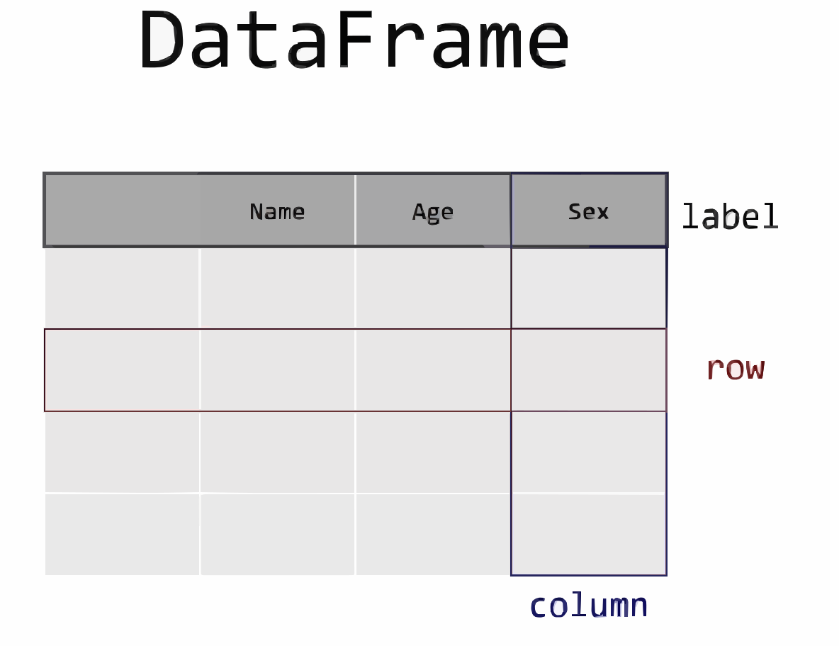
Let’s start with the absolute basics. The most basic polars object is DataFrame. A DataFrame is a 2-dimensional data structure that can store data of different types (including characters, integers, floating point values, categorical data, even lists) in columns. It is made up of rows and columns (with each row-column cell containing a value), plus contextual information: column names (which carry information about each column).

Note

Note: If you’re coming from pandas, be aware that polars does not use an index column and each row is indexed by its integer position in the table.

df = pl.DataFrame(
    data={
        "col0": [0, 0, 0, 0],
        "col1": [0, 0, 0, 0],
        "col2": [0, 0, 0, 0],
        "col3": ["a", "b", "b", "a"],
        "col4": ["alpha", "gamma", "gamma", "gamma"],
    },
)
df.head()

shape: (4, 5)

col0	col1	col2	col3	col4
i64	i64	i64	str	str
0	0	0	"a"	"alpha"
0	0	0	"b"	"gamma"
0	0	0	"b"	"gamma"
0	0	0	"a"	"gamma"

You can see there are 5 columns (named "col0" to "col4").

A second key point you should know is that the operations on a polars data frame can be chained together. We need not perform one assignment per line of code; we can actually do multiple assignments in a single command.

Let’s see an example of this. We’re going to string together four operations:

1. we will use filter() to find only the rows where the destination "dest" column has the value "IAH". We use the pl.col() expression to select the column for filtering condition. In effect, this step removes rows we’re not interested in.
2. we will use group_by() to group rows by the year, month, and day (we pass a list of columns to the group_by() function).
3. we will choose which columns to perform aggregation on after the group_by() operation by using the pl.col() expression inside agg(), to select the column. Here we just want one column, "arr_delay". In effect, this step removes columns we’re not interested in.
4. finally, we must specify what agg() operation we wish to apply; when aggregating the information in multiple rows down to one row, we need to say how that information should be aggregated. In this case, we’ll use the mean(). In effect, this step applies a statistic to the variable(s) we selected earlier, across the groups we created earlier.

flights.filter(pl.col("dest") == "IAH").group_by(["year", "month", "day"]).agg(
    pl.col("arr_delay").mean()
)

shape: (365, 4)

year	month	day	arr_delay
i64	i64	i64	f64
2013	1	25	-10.368421
2013	4	27	-4.5625
2013	4	15	2.954545
2013	1	9	18.055556
2013	10	24	2.809524
…	…	…	…
2013	9	12	50.3125
2013	7	20	-1.5
2013	1	18	-5.210526
2013	10	12	-13.866667
2013	10	2	-19.47619

You can see here that we’ve created a new data frame. To do it, we used three key operations:

1. manipulating rows
2. manipulating columns
3. applying statistics

Most operations you could want to do to a single data frame are covered by these, but there are different options for each of them depending on what you need.

Let’s now dig a bit more into these operations.

Manipulating Rows in Data Frames

Let’s create some fake data to show how this works.

import numpy as np

df = pl.DataFrame(
    data=np.reshape(range(36), (6, 6)),
    schema=["col" + str(i) for i in range(6)],
)
df.insert_column(
    6, pl.Series("col6", ["apple", "orange", "pineapple", "mango", "kiwi", "lemon"])
)
df

shape: (6, 7)

col0	col1	col2	col3	col4	col5	col6
i64	i64	i64	i64	i64	i64	str
0	1	2	3	4	5	"apple"
6	7	8	9	10	11	"orange"
12	13	14	15	16	17	"pineapple"
18	19	20	21	22	23	"mango"
24	25	26	27	28	29	"kiwi"
30	31	32	33	34	35	"lemon"

Accessing Rows

To access a particular row directly, you can get that by index (location in the data) or predicate/expression using .row(), which returns as a tuple. Remember that Python indices begin from zero, so to retrieve the first row by index you would use .row(0):

For example,

# Gets the first row of the DataFrame
df.row(0)

# Gets the fifth row of the DataFrame
df.row(4)

(24, 25, 26, 27, 28, 29, 'kiwi')

We can also access particular rows based on a predicate using .row() with the by_predicate parameter.

df.row(by_predicate=pl.col("col6") == "mango")

(18, 19, 20, 21, 22, 23, 'mango')

To get the row as a dictionary instead of a tuple with a mapping of column names to row values, specify named=True

# Get the first row of the DataFrame as a dictionary
df.row(0, named=True)

# Get the row where col6 is "mango" as a dictionary
df.row(by_predicate=pl.col("col6") == "mango", named=True)

{'col0': 18,
 'col1': 19,
 'col2': 20,
 'col3': 21,
 'col4': 22,
 'col5': 23,
 'col6': 'mango'}

We can also access rows using the .slice() function. As the function name implies, we get a slice of the DataFrame. we can use this to get a single row or a number of rows. To use this, we give it an offset - a start index, negative indexing is supported to index from the bottom of the DataFrame - and a length of the slice. This returns a DataFrame

df.slice(-2, 2)

shape: (2, 7)

col0	col1	col2	col3	col4	col5	col6
i64	i64	i64	i64	i64	i64	str
24	25	26	27	28	29	"kiwi"
30	31	32	33	34	35	"lemon"

Filtering rows

As with the flights example, we can also filter rows based on a condition using filter():

df.filter((pl.col("col6") == "kiwi") | (pl.col("col6") == "pineapple"))

shape: (2, 7)

col0	col1	col2	col3	col4	col5	col6
i64	i64	i64	i64	i64	i64	str
12	13	14	15	16	17	"pineapple"
24	25	26	27	28	29	"kiwi"

For numbers, you can also use the greater than and less than signs:

df.filter(pl.col("col0") > 6)

shape: (4, 7)

col0	col1	col2	col3	col4	col5	col6
i64	i64	i64	i64	i64	i64	str
12	13	14	15	16	17	"pineapple"
18	19	20	21	22	23	"mango"
24	25	26	27	28	29	"kiwi"
30	31	32	33	34	35	"lemon"

In fact, there are lots of options that work with filter(): as well as > (greater than), you can use >= (greater than or equal to), < (less than), <= (less than or equal to), == (equal to), and != (not equal to). You can also use operators & as well as | to combine multiple conditions. Here’s an example of & from the flights data frame:

# Flights that departed on January 1
flights.filter((pl.col("month") == 1) & (pl.col("day") <= 5))

shape: (4_334, 19)

year	month	day	dep_time	sched_dep_time	dep_delay	arr_time	sched_arr_time	arr_delay	carrier	flight	tailnum	origin	dest	air_time	distance	hour	minute	time_hour
i64	i64	i64	i64	i64	i64	i64	i64	i64	str	i64	str	str	str	i64	i64	i64	i64	str
2013	1	1	517	515	2	830	819	11	"UA"	1545	"N14228"	"EWR"	"IAH"	227	1400	5	15	"2013-01-01T10:00:00Z"
2013	1	1	533	529	4	850	830	20	"UA"	1714	"N24211"	"LGA"	"IAH"	227	1416	5	29	"2013-01-01T10:00:00Z"
2013	1	1	542	540	2	923	850	33	"AA"	1141	"N619AA"	"JFK"	"MIA"	160	1089	5	40	"2013-01-01T10:00:00Z"
2013	1	1	544	545	-1	1004	1022	-18	"B6"	725	"N804JB"	"JFK"	"BQN"	183	1576	5	45	"2013-01-01T10:00:00Z"
2013	1	1	554	600	-6	812	837	-25	"DL"	461	"N668DN"	"LGA"	"ATL"	116	762	6	0	"2013-01-01T11:00:00Z"
…	…	…	…	…	…	…	…	…	…	…	…	…	…	…	…	…	…	…
2013	1	5	2355	2359	-4	425	442	-17	"B6"	707	"N583JB"	"JFK"	"SJU"	193	1598	23	59	"2013-01-06T04:00:00Z"
2013	1	5	2357	2359	-2	432	437	-5	"B6"	727	"N649JB"	"JFK"	"BQN"	195	1576	23	59	"2013-01-06T04:00:00Z"
2013	1	5	null	1400	null	null	1518	null	"EV"	5712	"N827AS"	"JFK"	"IAD"	null	228	14	0	"2013-01-05T19:00:00Z"
2013	1	5	null	840	null	null	1001	null	"9E"	3422	null	"JFK"	"BOS"	null	187	8	40	"2013-01-05T13:00:00Z"
2013	1	5	null	1430	null	null	1735	null	"AA"	883	"N544AA"	"EWR"	"DFW"	null	1372	14	30	"2013-01-05T19:00:00Z"

Note that equality is tested by == and not by =, because the latter is used for assignment.

Re-arranging Rows

Again and again, you will want to re-order the rows of your data frame according to the values in a particular column. polars makes this very easy via the .sort() function. You can sort by single or multiple column names and also by expressions. If you provide more than one column name, each additional column will be used to break ties in the values of preceding columns. For example, the following code sorts by the departure time, which is spread over four columns.

flights.sort("dep_time")

shape: (336_776, 19)

year	month	day	dep_time	sched_dep_time	dep_delay	arr_time	sched_arr_time	arr_delay	carrier	flight	tailnum	origin	dest	air_time	distance	hour	minute	time_hour
i64	i64	i64	i64	i64	i64	i64	i64	i64	str	i64	str	str	str	i64	i64	i64	i64	str
2013	1	1	null	1630	null	null	1815	null	"EV"	4308	"N18120"	"EWR"	"RDU"	null	416	16	30	"2013-01-01T21:00:00Z"
2013	1	1	null	1935	null	null	2240	null	"AA"	791	"N3EHAA"	"LGA"	"DFW"	null	1389	19	35	"2013-01-02T00:00:00Z"
2013	1	1	null	1500	null	null	1825	null	"AA"	1925	"N3EVAA"	"LGA"	"MIA"	null	1096	15	0	"2013-01-01T20:00:00Z"
2013	1	1	null	600	null	null	901	null	"B6"	125	"N618JB"	"JFK"	"FLL"	null	1069	6	0	"2013-01-01T11:00:00Z"
2013	1	2	null	1540	null	null	1747	null	"EV"	4352	"N10575"	"EWR"	"CVG"	null	569	15	40	"2013-01-02T20:00:00Z"
…	…	…	…	…	…	…	…	…	…	…	…	…	…	…	…	…	…	…
2013	7	28	2400	2359	1	411	344	27	"B6"	1503	"N503JB"	"JFK"	"SJU"	204	1598	23	59	"2013-07-29T03:00:00Z"
2013	8	10	2400	2245	75	110	1	69	"B6"	234	"N328JB"	"JFK"	"BTV"	53	266	22	45	"2013-08-11T02:00:00Z"
2013	8	20	2400	2359	1	354	350	4	"B6"	745	"N708JB"	"JFK"	"PSE"	201	1617	23	59	"2013-08-21T03:00:00Z"
2013	9	2	2400	2359	1	411	340	31	"B6"	839	"N828JB"	"JFK"	"BQN"	217	1576	23	59	"2013-09-03T03:00:00Z"
2013	9	12	2400	2000	240	203	2230	213	"DL"	1147	"N910DE"	"LGA"	"ATL"	101	762	20	0	"2013-09-13T00:00:00Z"

# Sort by multiple columns by passing a list of columns.
flights.sort(["year", "month", "day", "dep_time"])

# Or use positional arguments to sort by multiple columns in the same way.
flights.sort("year", "month", "day", "dep_time")

shape: (336_776, 19)

year	month	day	dep_time	sched_dep_time	dep_delay	arr_time	sched_arr_time	arr_delay	carrier	flight	tailnum	origin	dest	air_time	distance	hour	minute	time_hour
i64	i64	i64	i64	i64	i64	i64	i64	i64	str	i64	str	str	str	i64	i64	i64	i64	str
2013	1	1	null	1935	null	null	2240	null	"AA"	791	"N3EHAA"	"LGA"	"DFW"	null	1389	19	35	"2013-01-02T00:00:00Z"
2013	1	1	null	1500	null	null	1825	null	"AA"	1925	"N3EVAA"	"LGA"	"MIA"	null	1096	15	0	"2013-01-01T20:00:00Z"
2013	1	1	null	1630	null	null	1815	null	"EV"	4308	"N18120"	"EWR"	"RDU"	null	416	16	30	"2013-01-01T21:00:00Z"
2013	1	1	null	600	null	null	901	null	"B6"	125	"N618JB"	"JFK"	"FLL"	null	1069	6	0	"2013-01-01T11:00:00Z"
2013	1	1	517	515	2	830	819	11	"UA"	1545	"N14228"	"EWR"	"IAH"	227	1400	5	15	"2013-01-01T10:00:00Z"
…	…	…	…	…	…	…	…	…	…	…	…	…	…	…	…	…	…	…
2013	12	31	2321	2250	31	46	8	38	"B6"	2002	"N179JB"	"JFK"	"BUF"	66	301	22	50	"2014-01-01T03:00:00Z"
2013	12	31	2328	2330	-2	412	409	3	"B6"	1389	"N651JB"	"EWR"	"SJU"	198	1608	23	30	"2014-01-01T04:00:00Z"
2013	12	31	2332	2245	47	58	3	55	"B6"	486	"N334JB"	"JFK"	"ROC"	60	264	22	45	"2014-01-01T03:00:00Z"
2013	12	31	2355	2359	-4	430	440	-10	"B6"	1503	"N509JB"	"JFK"	"SJU"	195	1598	23	59	"2014-01-01T04:00:00Z"
2013	12	31	2356	2359	-3	436	445	-9	"B6"	745	"N665JB"	"JFK"	"PSE"	200	1617	23	59	"2014-01-01T04:00:00Z"

You can use the keyword argument descending=True to re-order by a column or columns in descending order. For example, this code shows the most delayed flights:

flights.sort("dep_delay", descending=True)

shape: (336_776, 19)

year	month	day	dep_time	sched_dep_time	dep_delay	arr_time	sched_arr_time	arr_delay	carrier	flight	tailnum	origin	dest	air_time	distance	hour	minute	time_hour
i64	i64	i64	i64	i64	i64	i64	i64	i64	str	i64	str	str	str	i64	i64	i64	i64	str
2013	1	1	null	1630	null	null	1815	null	"EV"	4308	"N18120"	"EWR"	"RDU"	null	416	16	30	"2013-01-01T21:00:00Z"
2013	1	1	null	1935	null	null	2240	null	"AA"	791	"N3EHAA"	"LGA"	"DFW"	null	1389	19	35	"2013-01-02T00:00:00Z"
2013	1	1	null	1500	null	null	1825	null	"AA"	1925	"N3EVAA"	"LGA"	"MIA"	null	1096	15	0	"2013-01-01T20:00:00Z"
2013	1	1	null	600	null	null	901	null	"B6"	125	"N618JB"	"JFK"	"FLL"	null	1069	6	0	"2013-01-01T11:00:00Z"
2013	1	2	null	1540	null	null	1747	null	"EV"	4352	"N10575"	"EWR"	"CVG"	null	569	15	40	"2013-01-02T20:00:00Z"
…	…	…	…	…	…	…	…	…	…	…	…	…	…	…	…	…	…	…
2013	1	29	1703	1730	-27	1947	1957	-10	"F9"	837	"N208FR"	"LGA"	"DEN"	250	1620	17	30	"2013-01-29T22:00:00Z"
2013	1	11	1900	1930	-30	2233	2243	-10	"DL"	1435	"N934DL"	"LGA"	"TPA"	139	1010	19	30	"2013-01-12T00:00:00Z"
2013	11	10	1408	1440	-32	1549	1559	-10	"EV"	5713	"N825AS"	"LGA"	"IAD"	52	229	14	40	"2013-11-10T19:00:00Z"
2013	2	3	2022	2055	-33	2240	2338	-58	"DL"	1715	"N612DL"	"LGA"	"MSY"	162	1183	20	55	"2013-02-04T01:00:00Z"
2013	12	7	2040	2123	-43	40	2352	48	"B6"	97	"N592JB"	"JFK"	"DEN"	265	1626	21	23	"2013-12-08T02:00:00Z"

flights.sort(["dep_delay", "arr_delay"], descending=[True, False])

shape: (336_776, 19)

year	month	day	dep_time	sched_dep_time	dep_delay	arr_time	sched_arr_time	arr_delay	carrier	flight	tailnum	origin	dest	air_time	distance	hour	minute	time_hour
i64	i64	i64	i64	i64	i64	i64	i64	i64	str	i64	str	str	str	i64	i64	i64	i64	str
2013	3	8	null	1800	null	null	1937	null	"UA"	1177	null	"LGA"	"ORD"	null	733	18	0	"2013-03-08T23:00:00Z"
2013	2	8	null	1659	null	null	1822	null	"UA"	531	null	"EWR"	"BOS"	null	200	16	59	"2013-02-08T21:00:00Z"
2013	8	13	null	1727	null	null	1941	null	"EV"	5892	"N16561"	"EWR"	"CVG"	null	569	17	27	"2013-08-13T21:00:00Z"
2013	8	13	null	1225	null	null	1338	null	"EV"	5897	"N15973"	"EWR"	"ORF"	null	284	12	25	"2013-08-13T16:00:00Z"
2013	9	30	null	840	null	null	1020	null	"MQ"	3531	"N839MQ"	"LGA"	"RDU"	null	431	8	40	"2013-09-30T12:00:00Z"
…	…	…	…	…	…	…	…	…	…	…	…	…	…	…	…	…	…	…
2013	1	29	1703	1730	-27	1947	1957	-10	"F9"	837	"N208FR"	"LGA"	"DEN"	250	1620	17	30	"2013-01-29T22:00:00Z"
2013	1	11	1900	1930	-30	2233	2243	-10	"DL"	1435	"N934DL"	"LGA"	"TPA"	139	1010	19	30	"2013-01-12T00:00:00Z"
2013	11	10	1408	1440	-32	1549	1559	-10	"EV"	5713	"N825AS"	"LGA"	"IAD"	52	229	14	40	"2013-11-10T19:00:00Z"
2013	2	3	2022	2055	-33	2240	2338	-58	"DL"	1715	"N612DL"	"LGA"	"MSY"	162	1183	20	55	"2013-02-04T01:00:00Z"
2013	12	7	2040	2123	-43	40	2352	48	"B6"	97	"N592JB"	"JFK"	"DEN"	265	1626	21	23	"2013-12-08T02:00:00Z"

You can of course combine all of the above row manipulations to solve more complex problems. For example, we could look for the top three destinations of the flights that were most delayed on arrival that left on roughly on time:

(
    flights.filter((pl.col("dep_delay") <= 10) & (pl.col("dep_delay") >= -10))
    .sort("arr_delay", descending=True)
    .head(3)
)

shape: (3, 19)

year	month	day	dep_time	sched_dep_time	dep_delay	arr_time	sched_arr_time	arr_delay	carrier	flight	tailnum	origin	dest	air_time	distance	hour	minute	time_hour
i64	i64	i64	i64	i64	i64	i64	i64	i64	str	i64	str	str	str	i64	i64	i64	i64	str
2013	1	1	1525	1530	-5	1934	1805	null	"MQ"	4525	"N719MQ"	"LGA"	"XNA"	null	1147	15	30	"2013-01-01T20:00:00Z"
2013	1	1	1740	1745	-5	2158	2020	null	"MQ"	4413	"N739MQ"	"LGA"	"XNA"	null	1147	17	45	"2013-01-01T22:00:00Z"
2013	1	2	1848	1840	8	2333	2151	null	"9E"	3325	"N920XJ"	"JFK"	"DFW"	null	1391	18	40	"2013-01-02T23:00:00Z"

Exercises

1. Find all flights that

   1. Had an arrival delay of two or more hours

   2. Flew to Houston ("IAH" or "HOU")

   3. Were operated by United, American, or Delta

   4. Departed in summer (July, August, and September)

   5. Arrived more than two hours late, but didn’t leave late

   6. Were delayed by at least an hour, but made up over 30 minutes in flight

2. Sort flights to find the flights with longest departure delays.

3. Sort flights to find the fastest flights

4. Which flights traveled the farthest?

5. Does it matter what order you used filter() and sort() in if you’re using both? Why/why not? Think about the results and how much work the functions would have to do.

Manipulating Columns

This section will show you how to apply various operations you may need to columns in your data frame.

Creating New Columns

Let’s now move on to creating new columns, either using new information or from existing columns. Given a data frame, df, creating a new column with the same value repeated is done by using .with_columns(), with an expression assigned to a column name. Here we use pl.lit() which returns an expression representing a literal value, 5 in our case.

df = df.with_columns(new_column0=pl.lit(5))
df

shape: (6, 8)

col0	col1	col2	col3	col4	col5	col6	new_column0
i64	i64	i64	i64	i64	i64	str	i32
0	1	2	3	4	5	"apple"	5
6	7	8	9	10	11	"orange"	5
12	13	14	15	16	17	"pineapple"	5
18	19	20	21	22	23	"mango"	5
24	25	26	27	28	29	"kiwi"	5
30	31	32	33	34	35	"lemon"	5

If we do the same operation again, but this time assigning a Series to the same column, it will overwrite what was already in that column. A Series repesents a single column in a Polars DataFrame. Let’s see this with an example where we put different values in each position by assigning a list to the new column.

df = df.with_columns(new_column0=pl.Series([0, 1, 2, 3, 4, 5]))
df

shape: (6, 8)

col0	col1	col2	col3	col4	col5	col6	new_column0
i64	i64	i64	i64	i64	i64	str	i64
0	1	2	3	4	5	"apple"	0
6	7	8	9	10	11	"orange"	1
12	13	14	15	16	17	"pineapple"	2
18	19	20	21	22	23	"mango"	3
24	25	26	27	28	29	"kiwi"	4
30	31	32	33	34	35	"lemon"	5

TipExercise

What happens if you try to use assignment where the right-hand side values are longer or shorter than the length of the data frame?

We can actually use .with_columns to create more than one new column:

df = df.with_columns(new_column1=pl.lit(5), new_column2=pl.lit(6))
df

shape: (6, 10)

col0	col1	col2	col3	col4	col5	col6	new_column0	new_column1	new_column2
i64	i64	i64	i64	i64	i64	str	i64	i32	i32
0	1	2	3	4	5	"apple"	0	5	6
6	7	8	9	10	11	"orange"	1	5	6
12	13	14	15	16	17	"pineapple"	2	5	6
18	19	20	21	22	23	"mango"	3	5	6
24	25	26	27	28	29	"kiwi"	4	5	6
30	31	32	33	34	35	"lemon"	5	5	6

Very often, you will want to create a new column or modify a column that is the result of an operation on existing columns. There are a couple of ways to do this. The ‘stand-alone’ method works in a similar way to what we’ve just seen except that we refer to the data frame on the right-hand side of the assignment statement too:

df.with_columns(new_column2=pl.col("col0") - pl.col("new_column0"))

shape: (6, 10)

col0	col1	col2	col3	col4	col5	col6	new_column0	new_column1	new_column2
i64	i64	i64	i64	i64	i64	str	i64	i32	i64
0	1	2	3	4	5	"apple"	0	5	0
6	7	8	9	10	11	"orange"	1	5	5
12	13	14	15	16	17	"pineapple"	2	5	10
18	19	20	21	22	23	"mango"	3	5	15
24	25	26	27	28	29	"kiwi"	4	5	20
30	31	32	33	34	35	"lemon"	5	5	25

We can use .alias() with an expression to assign column names, when creating new columns. We can chain multiple expressions together with .with_columns(), which would create multiple new columns with the names assigned to .alias().

flights.with_columns(
    (pl.col("dep_delay") - pl.col("arr_delay")).alias("gain"),
    (pl.col("distance") / pl.col("air_time") * 60).alias("speed"),
)

shape: (336_776, 21)

year	month	day	dep_time	sched_dep_time	dep_delay	arr_time	sched_arr_time	arr_delay	carrier	flight	tailnum	origin	dest	air_time	distance	hour	minute	time_hour	gain	speed
i64	i64	i64	i64	i64	i64	i64	i64	i64	str	i64	str	str	str	i64	i64	i64	i64	str	i64	f64
2013	1	1	517	515	2	830	819	11	"UA"	1545	"N14228"	"EWR"	"IAH"	227	1400	5	15	"2013-01-01T10:00:00Z"	-9	370.044053
2013	1	1	533	529	4	850	830	20	"UA"	1714	"N24211"	"LGA"	"IAH"	227	1416	5	29	"2013-01-01T10:00:00Z"	-16	374.273128
2013	1	1	542	540	2	923	850	33	"AA"	1141	"N619AA"	"JFK"	"MIA"	160	1089	5	40	"2013-01-01T10:00:00Z"	-31	408.375
2013	1	1	544	545	-1	1004	1022	-18	"B6"	725	"N804JB"	"JFK"	"BQN"	183	1576	5	45	"2013-01-01T10:00:00Z"	17	516.721311
2013	1	1	554	600	-6	812	837	-25	"DL"	461	"N668DN"	"LGA"	"ATL"	116	762	6	0	"2013-01-01T11:00:00Z"	19	394.137931
…	…	…	…	…	…	…	…	…	…	…	…	…	…	…	…	…	…	…	…	…
2013	9	30	null	1455	null	null	1634	null	"9E"	3393	null	"JFK"	"DCA"	null	213	14	55	"2013-09-30T18:00:00Z"	null	null
2013	9	30	null	2200	null	null	2312	null	"9E"	3525	null	"LGA"	"SYR"	null	198	22	0	"2013-10-01T02:00:00Z"	null	null
2013	9	30	null	1210	null	null	1330	null	"MQ"	3461	"N535MQ"	"LGA"	"BNA"	null	764	12	10	"2013-09-30T16:00:00Z"	null	null
2013	9	30	null	1159	null	null	1344	null	"MQ"	3572	"N511MQ"	"LGA"	"CLE"	null	419	11	59	"2013-09-30T15:00:00Z"	null	null
2013	9	30	null	840	null	null	1020	null	"MQ"	3531	"N839MQ"	"LGA"	"RDU"	null	431	8	40	"2013-09-30T12:00:00Z"	null	null

Accessing Columns

Just as with selecting rows, there are many options and ways to select the columns to operate on. The one with the simplest syntax is the name of the data frame followed by square brackets and the column name (as a string)

df["col0"]

shape: (6,)

col0
i64
0
6
12
18
24
30

If you need to select multiple columns, you cannot just pass a string into df[...]; instead you need to pass an object that is iterable (and so have multiple items). The most straight forward way to select multiple columns is to pass a list. Remember, lists comes in square brackets so we’re going to see something with repeated square brackets: one for accessing the data frame’s innards and one for the list.

df[["col0", "new_column0", "col2"]]

shape: (6, 3)

col0	new_column0	col2
i64	i64	i64
0	0	2
6	1	8
12	2	14
18	3	20
24	4	26
30	5	32

We can also use .select() on the data frame to select columns, passing a single string to select a single column or an iterable, like a list, positional arguments or keyword arguments, to select multiple columns. Using keyword arguments renames the columns in the output

# selecting a single column
df.select("col0")

# Using positional arguments to select multiple columns
df.select("col0", "new_column0", "col2")

# Using keyword arguments to rename columns in the output
df.select(col1="col0", col2="new_column0", col3="col2")

shape: (6, 3)

col1	col2	col3
i64	i64	i64
0	0	2
6	1	8
12	2	14
18	3	20
24	4	26
30	5	32

Expressions are also accepted

df.select(pl.col("col0"), pl.col("new_column0") + 2, pl.col("col2") * 2)

shape: (6, 3)

col0	new_column0	col2
i64	i64	i64
0	2	4
6	3	16
12	4	28
18	5	40
24	6	52
30	7	64

If we want to access particular rows at the same time, we can chain .filter() or .slice() to the .select() function:

df.select("col0", "new_column0", "col2").slice(0, 2)

shape: (2, 3)

col0	new_column0	col2
i64	i64	i64
0	0	2
6	1	8

Sometimes, we’ll want to select columns based on the type of data that they hold. For this, we can call polars data types with an expression inside .select(). Let’s use this to select all columns with integers in the flights data.

flights.select(pl.col(pl.Int64))

shape: (336_776, 14)

year	month	day	dep_time	sched_dep_time	dep_delay	arr_time	sched_arr_time	arr_delay	flight	air_time	distance	hour	minute
i64	i64	i64	i64	i64	i64	i64	i64	i64	i64	i64	i64	i64	i64
2013	1	1	517	515	2	830	819	11	1545	227	1400	5	15
2013	1	1	533	529	4	850	830	20	1714	227	1416	5	29
2013	1	1	542	540	2	923	850	33	1141	160	1089	5	40
2013	1	1	544	545	-1	1004	1022	-18	725	183	1576	5	45
2013	1	1	554	600	-6	812	837	-25	461	116	762	6	0
…	…	…	…	…	…	…	…	…	…	…	…	…	…
2013	9	30	null	1455	null	null	1634	null	3393	null	213	14	55
2013	9	30	null	2200	null	null	2312	null	3525	null	198	22	0
2013	9	30	null	1210	null	null	1330	null	3461	null	764	12	10
2013	9	30	null	1159	null	null	1344	null	3572	null	419	11	59
2013	9	30	null	840	null	null	1020	null	3531	null	431	8	40

polars also provides a selectors module that we can use to select columns based on both data types and criteria such as patterns in the name of the column.

import polars.selectors as S

# Select all integer columns
flights.select(S.integer())

# Exclude string columns
flights.select(S.exclude(S.string()))

shape: (336_776, 14)

year	month	day	dep_time	sched_dep_time	dep_delay	arr_time	sched_arr_time	arr_delay	flight	air_time	distance	hour	minute
i64	i64	i64	i64	i64	i64	i64	i64	i64	i64	i64	i64	i64	i64
2013	1	1	517	515	2	830	819	11	1545	227	1400	5	15
2013	1	1	533	529	4	850	830	20	1714	227	1416	5	29
2013	1	1	542	540	2	923	850	33	1141	160	1089	5	40
2013	1	1	544	545	-1	1004	1022	-18	725	183	1576	5	45
2013	1	1	554	600	-6	812	837	-25	461	116	762	6	0
…	…	…	…	…	…	…	…	…	…	…	…	…	…
2013	9	30	null	1455	null	null	1634	null	3393	null	213	14	55
2013	9	30	null	2200	null	null	2312	null	3525	null	198	22	0
2013	9	30	null	1210	null	null	1330	null	3461	null	764	12	10
2013	9	30	null	1159	null	null	1344	null	3572	null	419	11	59
2013	9	30	null	840	null	null	1020	null	3531	null	431	8	40

# Select columns that contain "delay" in their name
flights.select(S.contains("delay"))

# Select columns that start with "arr"
flights.select(S.starts_with("arr"))

shape: (336_776, 2)

arr_time	arr_delay
i64	i64
830	11
850	20
923	33
1004	-18
812	-25
…	…
null	null
null	null
null	null
null	null
null	null

Other selectors commands include ends_with(), by_index(), first(), last(), duration(), numeric(), boolean() and more

Renaming Columns

We use the dedicated rename() function with a mapping, such as a dictionary or a lambda function. Dictionaries in Python consist of curly brackets with comma separated pairs of values where the first values maps into the second value. An example of a dictionary would be {'old_col1': 'new_col1', 'old_col2': 'new_col2'}. Let’s see this in practice (but note that we are not ‘saving’ the resulting data frame, just showing it—to save it, you’d need to add df = to the left-hand side of the code below).

df.rename({"col3": "letters", "col4": "names", "col6": "fruit"})

shape: (6, 10)

col0	col1	col2	letters	names	col5	fruit	new_column0	new_column1	new_column2
i64	i64	i64	i64	i64	i64	str	i64	i32	i32
0	1	2	3	4	5	"apple"	0	5	6
6	7	8	9	10	11	"orange"	1	5	6
12	13	14	15	16	17	"pineapple"	2	5	6
18	19	20	21	22	23	"mango"	3	5	6
24	25	26	27	28	29	"kiwi"	4	5	6
30	31	32	33	34	35	"lemon"	5	5	6

Using a lambda function, maps each column name as its argument, which you can then perform an operation on.

df.rename(lambda column_name: column_name.upper())

shape: (6, 10)

COL0	COL1	COL2	COL3	COL4	COL5	COL6	NEW_COLUMN0	NEW_COLUMN1	NEW_COLUMN2
i64	i64	i64	i64	i64	i64	str	i64	i32	i32
0	1	2	3	4	5	"apple"	0	5	6
6	7	8	9	10	11	"orange"	1	5	6
12	13	14	15	16	17	"pineapple"	2	5	6
18	19	20	21	22	23	"mango"	3	5	6
24	25	26	27	28	29	"kiwi"	4	5	6
30	31	32	33	34	35	"lemon"	5	5	6

Tip

A lambda function is a small, anonymous function in Python that performs a single operation. It’s a shorthand way to create a function without using def.

Re-ordering Columns

By default, new columns are added to the right-hand side of the data frame. But you may have reasons to want the columns to appear in a particular order, or perhaps you’d just find it more convenient to have new columns on the left-hand side when there are many columns in a data frame (which happens a lot).

The simplest way to re-order (all) columns is to create a new list of their names with them in the order that you’d like them: but be careful you don’t forget any columns that you’d like to keep!

Let’s see an example with a fresh version of the fake data from earlier. We’ll put all of the odd-numbered columns first, in descending order, then the even similarly using .select().

df = pl.DataFrame(
    data=np.reshape(range(36), (6, 6)), schema=["col" + str(i) for i in range(6)]
)
df

shape: (6, 6)

col0	col1	col2	col3	col4	col5
i64	i64	i64	i64	i64	i64
0	1	2	3	4	5
6	7	8	9	10	11
12	13	14	15	16	17
18	19	20	21	22	23
24	25	26	27	28	29
30	31	32	33	34	35

df = df.select(["col5", "col3", "col1", "col4", "col2", "col0"])
df

shape: (6, 6)

col5	col3	col1	col4	col2	col0
i64	i64	i64	i64	i64	i64
5	3	1	4	2	0
11	9	7	10	8	6
17	15	13	16	14	12
23	21	19	22	20	18
29	27	25	28	26	24
35	33	31	34	32	30

Of course, this is quite tedious if you have lots of columns! There are methods that can help make this easier depending on your context. Perhaps you’d just liked to sort the columns in order? This can be achieved by combining sorted() and the .select() function, passing the DataFrame .columns.

# Alphabetical order
df.select(sorted(df.columns))

# Reverse alphabetical order
df.select(sorted(df.columns, reverse=True))

shape: (6, 6)

col5	col4	col3	col2	col1	col0
i64	i64	i64	i64	i64	i64
5	4	3	2	1	0
11	10	9	8	7	6
17	16	15	14	13	12
23	22	21	20	19	18
29	28	27	26	25	24
35	34	33	32	31	30

Column and Row Exercises

1. Compare air_time with arr_time - dep_time. What do you expect to see? What do you see? What do you need to do to fix it?

2. Compare dep_time, sched_dep_time, and dep_delay. How would you expect those three numbers to be related?

3. Brainstorm as many ways as possible to select dep_time, dep_delay, arr_time, and arr_delay from flights.

4. What happens if you include the name of a row or column multiple times when trying to select them?

Grouping and applying summary statistics

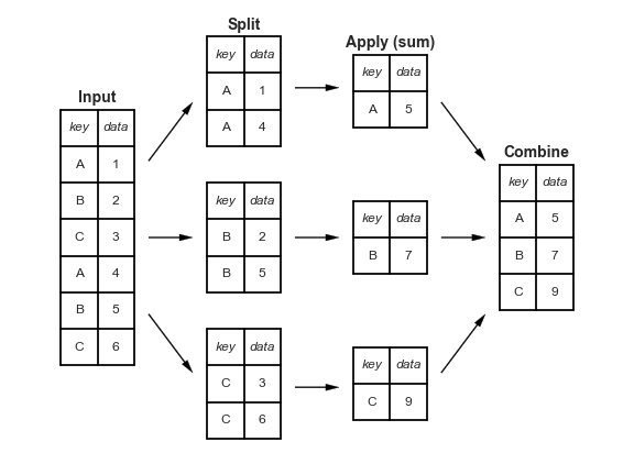
So far you’ve learned about working with rows and columns. polars gets even more powerful when you add in the ability to work with groups. And because groups tend to imply an aggregation or pooling of data, they go hand-in-glove with the application of a summary statistic.

The diagram below gives a sense of how these operations can proceed together. Note that the ‘split’ operation is achieved through grouping, while apply produces summary statistics. At the end, you get a data frame with a new index (one entry per group) in what is shown as the ‘combine’ step.

Grouping and Aggregating

Let’s take a look at creating a group using the .group_by() function, then followed by the .agg() function for aggregation, selecting a column and applying a summary statistic via an aggregation.

flights.group_by("month").agg(pl.col("dep_delay").mean())

shape: (12, 2)

month	dep_delay
i64	f64
9	6.722476
3	13.227076
12	16.576688
11	5.435362
6	20.846332
…	…
10	6.243988
8	12.61104
5	12.986859
7	21.727787
1	10.036665

This now represents the mean departure delay by month. The mechanics happenning here is that the DataFrame is grouped by each unique item in the “month” column and then a mean summary statistic is derived on the “dep_delay” column from each group.

Other summary statistics can be derived from aggregations. Some common options are in the table below:

Aggregation	Description
count()	Number of non-null items
len()	Number of all items
first(), last()	First and last item
mean(), median()	Mean and median
min(), max()	Minimum and maximum
std(), var()	Standard deviation and variance
mad()	Mean absolute deviation
product()	Product of all items
sum()	Sum of all items
value_counts()	Counts of unique values

For doing multiple aggregations on multiple columns with new names for the output variables, the syntax becomes

# Multiple aggregations using polars' syntactic sugar (shorthand) for mean and count
flights.group_by("month").agg(
    mean_delay=pl.mean("dep_delay"),
    count_flights=pl.count("dep_delay"),
)

shape: (12, 3)

month	mean_delay	count_flights
i64	f64	u32
9	6.722476	27122
12	16.576688	27110
3	13.227076	27973
6	20.846332	27234
1	10.036665	26483
…	…	…
4	13.938038	27662
2	10.816843	23690
5	12.986859	28233
11	5.435362	27035
8	12.61104	28841

Means and counts can get you a surprisingly long way in data science!

Grouping by multiple variables

This is as simple as passing .group_by() a list or multiple strings representing columns instead of a single string representing a single column.

month_year_delay = flights.group_by("month", "year").agg(
    mean_delay=pl.mean("dep_delay"),
    count_flights=pl.count("dep_delay"),
)
month_year_delay

shape: (12, 4)

month	year	mean_delay	count_flights
i64	i64	f64	u32
5	2013	12.986859	28233
9	2013	6.722476	27122
10	2013	6.243988	28653
8	2013	12.61104	28841
6	2013	20.846332	27234
…	…	…	…
12	2013	16.576688	27110
7	2013	21.727787	28485
3	2013	13.227076	27973
2	2013	10.816843	23690
1	2013	10.036665	26483

Groupby Exercises

1. Which carrier has the worst delays? Challenge: can you disentangle the effects of bad airports vs. bad carriers? Why/why not? (Hint: think about flights.group_by(["carrier", "dest"]))

2. Find the most delayed flight to each destination.

3. How do delays vary over the course of the day?